TEL:+86 132 6656 7067


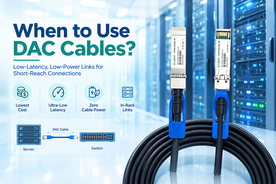
Direct Attach Copper (DAC) cables are the workhorse of short-reach data center interconnect. They are the lowest-cost, lowest-latency, and lowest-power option for connecting servers, switches, storage arrays, and GPU nodes within a rack or between adjacent racks. For decades, DAC has been the default choice for Top-of-Rack (ToR) links, and even in the era of 800G and 1.6T networking, passive copper remains the first option to evaluate whenever distance permits.
But DAC is not a universal solution. Its reach is fundamentally limited by copper's frequency-dependent attenuation, and that limit shrinks dramatically as lane rates climb. At 25G NRZ, passive DAC can span 5 meters. At 100G PAM4 per lane, the practical limit falls to 2–3 meters, and at 200G PAM4 per lane for 1.6T, it drops to roughly 1 meter. Understanding where DAC fits—and where it must give way to Active Electrical Cables (AEC), Active Optical Cables (AOC), or pluggable optics—is essential for building efficient, reliable AI data center networks.
This guide examines the technical foundations of DAC cables, the distinction between passive and active variants, the scenarios where DAC wins, and the design trade-offs that determine when copper remains viable and when it does not.
1. What Is a DAC Cable?
A DAC cable is a factory-terminated twinaxial copper assembly with integrated connector modules that plug directly into standard switch, server, or storage ports. The connectors have the same form factor as optical transceivers—SFP+, SFP28, QSFP+, QSFP28, QSFP-DD, OSFP, and OSFP-XD—but they are permanently attached to the copper cable and cannot be removed like a pluggable module.
The cable itself is built around twinaxial construction: two parallel or lightly twisted copper conductors carrying differential signals, individually insulated, wrapped in a metallic shield, and enclosed in an outer protective jacket.This differential signaling architecture is the foundation of DAC's EMI immunity. External electromagnetic noise couples equally onto both conductors and is cancelled during differential demodulation at the receiver, allowing stable high-speed transmission in dense, electrically noisy cabinet environments.
Because DAC transmits electrical signals directly without optical-electrical-optical (O-E-O) conversion, it eliminates the latency and power overhead associated with optical transceivers. A passive DAC link adds essentially zero active power and sub-nanosecond latency per meter, making it the most efficient interconnect option for the distances it can support.
2. Passive DAC vs. Active DAC
DAC cables fall into two primary categories based on whether they contain active electronics for signal conditioning.
2.1 Passive DAC
A passive DAC contains no electronic components in its connector modules. It relies entirely on the copper medium and the host SerDes to transmit and receive signals. This simplicity yields several advantages:
Zero active power consumption — no power is drawn by the cable itself.
Lowest cost per link — no signal-conditioning chips or equalizers.
Highest reliability — fewer active components means fewer failure points.
Lowest latency — direct electrical transmission with no processing delay.
The trade-off is reach. Passive DAC is limited to approximately 7 meters at lower speeds, but that limit contracts sharply as data rates increase. At 400G (8×50G PAM4), passive DAC reach is roughly 3 meters. At 800G (8×100G PAM4), it falls to about 2 meters. At 1.6T (8×200G PAM4), practical reach is approximately 1 meter.
2.2 Active DAC (ACC)
Active DAC, also called Active Copper Cable (ACC), incorporates signal-conditioning electronics—typically linear equalizers—in the connector modules. These components compensate for channel loss and extend reach beyond passive limits.
Active DAC typically achieves 5–10 meters of reach depending on data rate and implementation, at the cost of higher power consumption and a higher price point than passive DAC. The active electronics consume a small amount of power (typically under 1 W per end), but this remains far below the power required by optical alternatives.
| Characteristic | Passive DAC | Active DAC (ACC) |
|---|---|---|
| Signal Conditioning | None | Linear equalizer in connector |
| Typical Reach (25G) | Up to 5–7 m | Up to 10–15 m |
| Typical Reach (400G) | ~3 m | ~5–7 m |
| Power Consumption | ~0 W | < 1 w per end |
| Cost | Lowest | Moderate |
| Best For | In-rack, cost-sensitive, latency-critical | Adjacent racks, reach-limited passive |
3. Where DAC Cables Win
DAC cables are the correct choice in a well-defined set of scenarios. The common thread is short distance, high port density, and sensitivity to cost or latency.
3.1 In-Rack Server-to-Switch Connections
The most common DAC deployment is connecting servers to a Top-of-Rack switch within the same cabinet. Distances in this scenario are typically 0.5–3 meters, well within passive DAC reach even at 400G and 800G rates. A 3-meter DAC for a ToR-to-server link is a standard deployment pattern, and at 400G/800G rates, passive DAC at 1–3 meters delivers the lowest cost and lowest latency per link.
Meta's AI cluster architecture uses DAC cables to connect rack training switches to GPUs, demonstrating DAC's viability in production AI infrastructure at scale.
3.2 Adjacent-Rack Connections
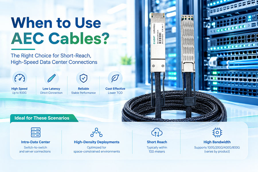
When links must cross between neighboring racks, distances may extend to 3–7 meters. Passive DAC can handle this range at lower speeds (25G, 50G), but at 100G per lane and above, active DAC or ACC becomes necessary to maintain signal integrity. AEC (Active Electrical Cable) extends copper reach further with integrated DSP, but at higher cost and power than ACC.
3.3 Latency-Critical Environments
DAC introduces no O-E-O conversion, no DSP processing latency, and no serialization delay beyond what the SerDes itself adds. For AI training clusters, high-frequency trading, and other latency-sensitive workloads, this makes DAC the preferred physical layer whenever distance permits. Direct copper links deliver minimal latency ideal for AI training and high-frequency trading.
3.4 Cost-Sensitive High-Density Deployments
In deployments with hundreds or thousands of short links—leaf-spine fabrics, storage clusters, GPU pod interconnects—DAC's cost advantage compounds rapidly. A passive DAC link may cost tens of dollars, while an equivalent AOC or optical module pair can cost several times more. For dense, short, high-count deployments, passive DAC yields the best total cost of ownership.
3.5 Breakout Applications
DAC breakout cables allow a single high-speed port to be split into multiple lower-speed ports. For example, a 400G QSFP-DD port can break out to four 100G ports, or an 800G OSFP port to two 400G ports. This is valuable for optimizing port density in ToR switches and connecting switches to servers with lower per-port bandwidth requirements. Breakout DAC cables enhance panel port density and transmit high data rates over short distances.
4. Where DAC Cables Reach Their Limits
DAC's limitations are equally well-defined. Recognizing when DAC is no longer the right choice prevents field failures, signal integrity problems, and hidden operational costs.
4.1 Distance Beyond Copper Reach
The fundamental constraint of DAC is copper's frequency-dependent attenuation. As lane rates increase, insertion loss at the Nyquist frequency rises, and the signal-to-noise ratio at the receiver degrades rapidly. Passive DAC that comfortably spans 5 meters at 25G NRZ may barely reach 1 meter at 200G PAM4 per lane for 1.6T. When the required link distance exceeds the achievable reach at the target data rate, DAC is no longer viable.
4.2 Cross-Aisle and Cross-Row Links
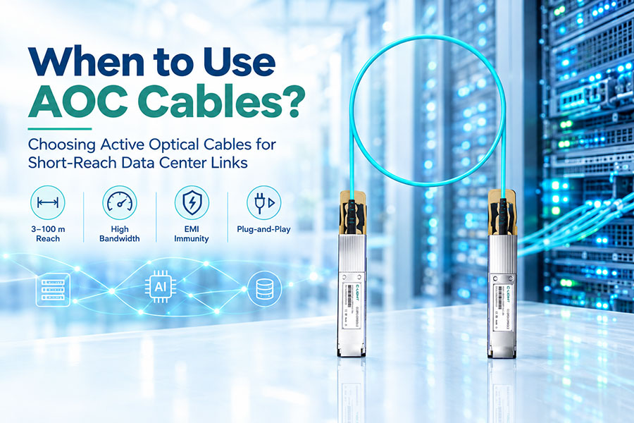
Distances beyond roughly 7 meters—cross-aisle connections, row-to-row links, aggregation switch uplinks—exceed copper's practical reach even with active DAC. In these scenarios, AOC or optical transceivers become necessary. Current deployment patterns use 3-meter DAC for ToR-to-server and 30–300-meter AOC for aggregation switch links.
4.3 High-EMI Environments
While twinax shielding provides good EMI immunity for most cabinet environments, extremely noisy industrial settings or areas with high-power radio frequency sources may still affect copper transmission. AOC, being immune to electromagnetic interference by nature, is preferred in such environments.
4.4 Cable Management and Airflow Constraints
Copper DAC cables are thicker, heavier, and less flexible than fiber AOCs. They have larger bend radii and occupy more space in cable trays and behind racks. In high-density deployments where airflow and cable routing are constrained, the bulk of copper cables can create thermal and management challenges that offset DAC's cost advantage. AOC is lighter and easier to deploy, effectively reducing cable congestion in data centers.
5. DAC vs. AOC: The Fundamental Trade-Off
The choice between DAC and AOC is the most common cabling decision in short-reach data center networking. Both support the same Ethernet and InfiniBand speeds—25G, 50G, 100G, 200G, 400G, and 800G—and use compatible connector form factors. The differences are in medium, reach, power, and cost.
| Characteristic | DAC (Copper Twinax) | AOC (Active Optical Cable) |
|---|---|---|
| Medium | Copper twinax | Multimode fiber |
| Typical Reach (25G–100G) | Passive: ≤5–7 m; Active: ≤15 m | 25–100 m |
| Typical Reach (400G/800G) | Passive: ≤3 m; Active: ≤5–7 m | 30–100 m |
| EMI Immunity | Good (shielded twinax) | Excellent (fiber is dielectric) |
| Power Consumption | Passive: ~0 W; Active:< 1 w | ~1 W per module (both ends) |
| Latency | Extremely low | Very low, slightly higher than DAC |
| Cable Size & Weight | Thick, heavy, less flexible | Thin, lightweight, flexible |
| Cost per Link | Lowest | Higher |
| Best For | In-rack, adjacent-rack, latency-critical | Cross-rack, high-EMI, cable-dense |
The decision rule is straightforward: use DAC for distances under 3 meters at high speeds (400G+), or under 7 meters at lower speeds (25G–100G), when cost and latency are priorities. Switch to AOC when distance exceeds DAC reach, when cable management is a constraint, or when the environment demands complete EMI immunity. DAC for short runs, AOC for long; DAC for cost, AOC for flexibility.
6. DAC Reach Shrinks as Data Rates Rise
One of the most important—and often underestimated—aspects of DAC selection is how reach contracts with each generation of Ethernet speed. The same copper cable that comfortably spans a rack at 25G may not reach across the same rack at 800G.
| Data Rate per Lane | Aggregate Example | Passive DAC Reach | Active DAC / AEC Reach |
|---|---|---|---|
| 25G NRZ | 100G (4 lanes) | Up to 5 m | Up to 15 m |
| 50G PAM4 | 400G (8 lanes) | Up to 3 m | Up to 5–7 m |
| 100G PAM4 | 800G (8 lanes) | Up to 2 m | Up to 3–5 m |
| 200G PAM4 | 1.6T (8 lanes) | ~1 m | ~2–3 m |
The contraction is dramatic. NVIDIA's passive DAC catalog reaches 5 meters at EDR 100G (25G NRZ), 2 meters at HDR 200G (50G PAM4), and only 0.5–1.5 meters at NDR 400G and 800G (100G PAM4). At 1.6T with 200G PAM4 per lane, passive DAC is effectively limited to links within a single rack unit or between immediately adjacent units.
This reach contraction means that network architects must re-evaluate DAC viability at every speed transition. A deployment that relied on 3-meter DACs at 100G may find that the same 3-meter distance requires AEC at 800G and AOC at 1.6T.
7. DAC, ACC, and AEC: The Copper Continuum
The copper interconnect landscape extends beyond passive and active DAC to include Active Electrical Cables (AEC), which bridge the gap between copper and optical solutions.
7.1 ACC: Linear Equalization
ACC (Active Copper Cable) uses linear equalizers at one or both ends of the cable to compensate for channel loss. It extends reach moderately beyond passive DAC—typically 5–7 meters at 400G—with low power consumption and moderate cost.
7.2 AEC: DSP-Based Signal Conditioning
AEC (Active Electrical Cable) incorporates full DSPs at one or both ends, providing more powerful equalization, retiming, and error correction than linear equalization alone. AEC achieves reaches of 5–15 meters or more, approaching AOC's range while retaining copper's cost and latency advantages for moderate distances.
AEC is positioned between DAC and AOC in cost and power. It consumes approximately half the power of AOC, making it an attractive option for deployments that need more reach than DAC provides but cannot justify the cost and power of optical links.
| Characteristic | Passive DAC | ACC (Active DAC) | AEC | AOC |
|---|---|---|---|---|
| Signal Processing | None | Linear equalizer | DSP | Optical DSP / retimer |
| Typical Reach (400G) | ≤3 m | 3–5 m | 5–7 m | 30–100 m |
| Power (per link, 400G) | ~0 W | ~1–2 W | <3 w=""> | ~5–8 W |
| Cost | Lowest | Low | Moderate | Highest (copper options) |
| Latency | Lowest | Very low | Low | Low |
| Best For | In-rack | Adjacent rack | Cross-rack within row | Cross-row, long reach |
The copper continuum—passive DAC, ACC, AEC—allows network designers to extend copper's reach as far as possible before resorting to optical solutions. Each step adds power, cost, and complexity, but each also adds distance capability that may be essential for the target topology.
8. DAC in AI Data Centers: Specific Considerations
AI workloads place unique demands on interconnect infrastructure. GPU clusters generate massive east-west traffic, training jobs are sensitive to latency and jitter, and the sheer number of links in a large AI cluster magnifies the cost and power impact of every cable decision.
8.1 GPU-to-Switch Connections
In AI clusters, each GPU node typically connects to a ToR switch via one or more high-speed links. These connections are almost always within a single rack or between immediately adjacent racks, making DAC the default choice. Meta's AI cluster architecture demonstrates this pattern, using DAC cables for rack training switch connections to GPUs.
At 400G per GPU port (NDR InfiniBand or 400G Ethernet), passive DAC at 0.5–1.5 meters is the standard. At 800G per port, passive DAC reach shrinks to approximately 1 meter, and careful rack layout—placing the switch and GPU nodes in the same or adjacent rack units—becomes essential to keep DAC viable.
8.2 Cable Density and Thermal Load
A large AI cluster may contain tens of thousands of DAC links. Each passive DAC link consumes essentially zero power, but the cables themselves occupy physical space and can impede airflow. The thermal benefit of DAC's zero active power is significant: every watt not consumed by a cable is a watt not requiring cooling. In dense GPU racks where thermal headroom is already constrained, passive DAC's zero-power operation is a meaningful advantage over AOC or optical modules.
8.3 Latency Sensitivity
AI training and inference workloads are sensitive to communication latency. DAC's direct electrical transmission eliminates the serialization and deserialization delays, optical conversion latency, and DSP processing latency associated with AOC and optical modules. For workloads where every nanosecond of collective communication latency matters, DAC provides the lowest-latency physical layer available for the distances it can support.
8.4 Reliability and Serviceability
Passive DAC has no active components in the cable or connectors. This simplicity translates directly to reliability: there is nothing to fail except the copper conductors and solder joints, both of which are extremely robust. Field failure rates for passive DAC are correspondingly low. When a failure does occur, replacement is straightforward: unplug and replace the entire cable. There is no module to remove, no fiber to clean, no optical alignment to worry about.
9. Evaluating DAC for a Specific Deployment
Selecting the right interconnect for a given link requires a structured evaluation of requirements against DAC capabilities.
| Evaluation Factor | What to Confirm |
|---|---|
| Link Distance | Physical cable path length, including service loops and slack |
| Data Rate per Lane | 25G, 50G, 100G, or 200G PAM4; determines passive reach limit |
| Connector Form Factor | SFP28, QSFP28, QSFP-DD, OSFP, OSFP-XD; must match host ports |
| Breakout Requirement | Whether one high-speed port needs to split to multiple lower-speed ports |
| Cable Management Space | Bend radius, tray capacity, airflow path interference |
| EMI Environment | Proximity to power cables, motors, RF sources |
| Latency Budget | Whether O-E-O conversion latency is acceptable |
| Power Budget | Whether active cable power is acceptable at scale |
| Cost per Link | Capital cost and total cost of ownership over deployment lifetime |
A disciplined evaluation compares passive DAC, active DAC/ACC, AEC, AOC, and optical module options for each link category in the network. In many cases, the optimal design uses a mix: passive DAC for the shortest in-rack links, active DAC or AEC for adjacent-rack connections, and AOC or optics for everything beyond copper's reach.
10. The Future of DAC in Higher-Speed Networks
As Ethernet advances toward 1.6T and eventually 3.2T, passive DAC reach continues to shrink. At 200G PAM4 per lane (1.6T), passive DAC is limited to approximately 1 meter. This is sufficient for connecting a switch ASIC to an immediately adjacent port or for very short intra-rack links, but it leaves little margin for cable routing or service loops.
The industry response has been to extend the copper ecosystem through ACC and AEC. These active copper cables push reach back to 2–3 meters at 1.6T and 5–7 meters at 800G, preserving copper's cost and latency advantages for a larger fraction of data center links. AEC in particular is emerging as the preferred solution for links that exceed passive DAC reach but do not require the full distance capability of optical cables.
For 3.2T, with 400G PAM4 per lane, passive DAC may be limited to sub-meter links, and even AEC reach may compress. At that point, optical solutions—whether AOC or co-packaged optics—will likely dominate all but the most trivial intra-rack connections.
But for the 400G, 800G, and 1.6T generations that dominate current AI data center deployments, DAC and its active copper extensions remain the most cost-effective and power-efficient interconnect for the majority of short-reach links. The key is knowing where those links are and designing the rack layout to keep distances within copper's reach.
11.Conclusion
DAC cables are the right choice for short-reach data center interconnect when distance, cost, latency, and power are the primary considerations. Passive DAC offers the lowest cost, lowest latency, and zero power consumption for links within a rack. Active DAC and AEC extend copper reach to adjacent racks, preserving copper's advantages where passive DAC can no longer span the required distance.
The critical constraint is reach, and that constraint tightens with every increase in lane rate. At 25G, passive DAC spans 5 meters. At 100G per lane, it spans 2 meters. At 200G per lane for 1.6T, it spans roughly 1 meter. Network designers must plan rack layouts with this contraction in mind, using the copper continuum—passive DAC, ACC, AEC—to maximize the fraction of links that avoid the cost and power of optical solutions.
When distance exceeds copper's reach, AOC or optical modules become necessary. But for the dense, short, high-count links that dominate AI data center topologies, DAC remains the most efficient answer. The question is not whether to use DAC, but where the distance boundary falls for each link in the network.
 >
>

 >
>
 >
>
 >
>
 >
>
 >
>
 >
>
 >
>